Tech Focus: Sound Suites and Acoustic Testing Booths
A product review of anechoic chambers and test suites.
Read More
A product review of anechoic chambers and test suites.
Read More
A field study on the accuracy of a new system for making direct real-ear-to-coupler difference (RECD) measurements in children.
Read More
A behind-the-scenes look at a few select companies and some of the people who make them successful.
Read More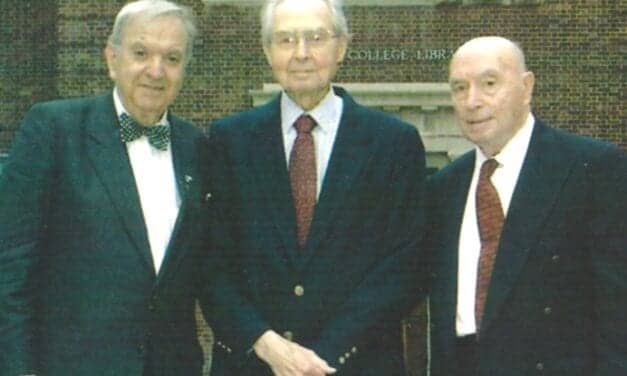
The legacy of Robert West, PhD, and the contributions made by a few of the many talented graduates of Brooklyn College.
Read More
Practical advice for converting the reluctant hearing-impaired visitor into your patient.
Read More
Serving as an expert witness in a legal trial can be professionally and personally rewarding. Here are some tips on what to expect and how to proceed.
Read Morerev.gif)
An introduction to ASSRs and their applications in a real-world fitting environment.
Read More
We need to routinely find the loudness discomfort levels of patients and fully define their residual hearing capabilities. Only then can we provide a truly customized fitting when moving onto items such as target gain, etc.
Read More